vignettes/ArchaeoChron.Rmd
ArchaeoChron.Rmd
## Load packages
library(ArchaeoChron)
library(ArchaeoPhases)
library(coda) # MCMC diagnostic
The sunspot data is constituted of several dates assumed to be contemporaneous of a single event. These dates do not need any calibration but their unit is in year before 2016.
Let’s first use a simple Bayesian model.
data(sunspot)
<- combination_Gauss(
MCMC1 M = sunspot$Age[1:5],
s = sunspot$Error[1:5],
refYear = rep(2016, 5),
studyPeriodMin = 900,
studyPeriodMax = 1500,
variable.names = c('theta')
)#> [1] "Update period"
#>
|
| | 0%
|
|* | 2%
|
|** | 4%
|
|*** | 6%
|
|**** | 8%
|
|***** | 10%
|
|****** | 12%
|
|******* | 14%
|
|******** | 16%
|
|********* | 18%
|
|********** | 20%
|
|*********** | 22%
|
|************ | 24%
|
|************* | 26%
|
|************** | 28%
|
|*************** | 30%
|
|**************** | 32%
|
|***************** | 34%
|
|****************** | 36%
|
|******************* | 38%
|
|******************** | 40%
|
|********************* | 42%
|
|********************** | 44%
|
|*********************** | 46%
|
|************************ | 48%
|
|************************* | 50%
|
|************************** | 52%
|
|*************************** | 54%
|
|**************************** | 56%
|
|***************************** | 58%
|
|****************************** | 60%
|
|******************************* | 62%
|
|******************************** | 64%
|
|********************************* | 66%
|
|********************************** | 68%
|
|*********************************** | 70%
|
|************************************ | 72%
|
|************************************* | 74%
|
|************************************** | 76%
|
|*************************************** | 78%
|
|**************************************** | 80%
|
|***************************************** | 82%
|
|****************************************** | 84%
|
|******************************************* | 86%
|
|******************************************** | 88%
|
|********************************************* | 90%
|
|********************************************** | 92%
|
|*********************************************** | 94%
|
|************************************************ | 96%
|
|************************************************* | 98%
|
|**************************************************| 100%
#> [1] "Acquire period"
#>
|
| | 0%
|
|* | 2%
|
|** | 4%
|
|*** | 6%
|
|**** | 8%
|
|***** | 10%
|
|****** | 12%
|
|******* | 14%
|
|******** | 16%
|
|********* | 18%
|
|********** | 20%
|
|*********** | 22%
|
|************ | 24%
|
|************* | 26%
|
|************** | 28%
|
|*************** | 30%
|
|**************** | 32%
|
|***************** | 34%
|
|****************** | 36%
|
|******************* | 38%
|
|******************** | 40%
|
|********************* | 42%
|
|********************** | 44%
|
|*********************** | 46%
|
|************************ | 48%
|
|************************* | 50%
|
|************************** | 52%
|
|*************************** | 54%
|
|**************************** | 56%
|
|***************************** | 58%
|
|****************************** | 60%
|
|******************************* | 62%
|
|******************************** | 64%
|
|********************************* | 66%
|
|********************************** | 68%
|
|*********************************** | 70%
|
|************************************ | 72%
|
|************************************* | 74%
|
|************************************** | 76%
|
|*************************************** | 78%
|
|**************************************** | 80%
|
|***************************************** | 82%
|
|****************************************** | 84%
|
|******************************************* | 86%
|
|******************************************** | 88%
|
|********************************************* | 90%
|
|********************************************** | 92%
|
|*********************************************** | 94%
|
|************************************************ | 96%
|
|************************************************* | 98%
|
|**************************************************| 100%
The output of the function combination_Gauss()
is a
Markov chain of the posterior distribution of the Bayesian model.
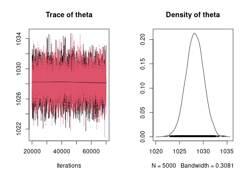
First, let’s check the convergence of the Markov chain of each parameter.
plot(MCMC1)
gelman.diag(MCMC1)
#> Potential scale reduction factors:
#>
#> Point est. Upper C.I.
#> theta 1 1
The Gelman diagnotic gives point estimates about 1, so convergence is reached.
Now, we can use the package ArchaeoPhases in order to describe the posterior distribution of the parameters.
Here we will focus on the posterior distribution of the date of interest, i.e. the parameter theta.
MCMCSample1 <- cbind(MCMC1[[1]], MCMC1[[2]])
MCMCEvent1 <- as_events(MCMCSample1, calendar = CE())
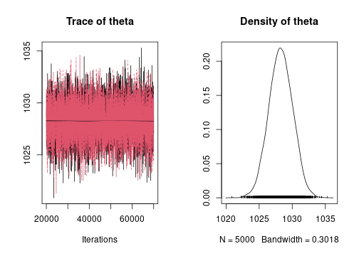
plot(MCMCEvent1[, 1], level = 0.95)
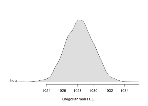
(M1 <- summary(MCMCEvent1[, 1], level = 0.95))
#> mad mean sd min q1 median q3 max start end
#> theta 1028 1028 3 1021 1027 1028 1029 1035 1025 1032
The date (mean posterior distribution) of the sunspot estimated using a simple Bayesian model that combines dates, is dates at 1028 years after Christ. This date is associated with a 95% confidence interval : [1025, 1032].
Let’s use the function
combinationWithOutliers_Gauss()
.
<- combinationWithOutliers_Gauss(
MCMC2 M = sunspot$Age[1:5],
s = sunspot$Error[1:5],
refYear = rep(2016, 5),
outliersIndivVariance = rep(1, 5),
outliersBernouilliProba = rep(0.2, 5),
studyPeriodMin = 800,
studyPeriodMax = 1500,
variable.names = c('theta')
)#> [1] "Update period"
#>
|
| | 0%
|
|* | 2%
|
|** | 4%
|
|*** | 6%
|
|**** | 8%
|
|***** | 10%
|
|****** | 12%
|
|******* | 14%
|
|******** | 16%
|
|********* | 18%
|
|********** | 20%
|
|*********** | 22%
|
|************ | 24%
|
|************* | 26%
|
|************** | 28%
|
|*************** | 30%
|
|**************** | 32%
|
|***************** | 34%
|
|****************** | 36%
|
|******************* | 38%
|
|******************** | 40%
|
|********************* | 42%
|
|********************** | 44%
|
|*********************** | 46%
|
|************************ | 48%
|
|************************* | 50%
|
|************************** | 52%
|
|*************************** | 54%
|
|**************************** | 56%
|
|***************************** | 58%
|
|****************************** | 60%
|
|******************************* | 62%
|
|******************************** | 64%
|
|********************************* | 66%
|
|********************************** | 68%
|
|*********************************** | 70%
|
|************************************ | 72%
|
|************************************* | 74%
|
|************************************** | 76%
|
|*************************************** | 78%
|
|**************************************** | 80%
|
|***************************************** | 82%
|
|****************************************** | 84%
|
|******************************************* | 86%
|
|******************************************** | 88%
|
|********************************************* | 90%
|
|********************************************** | 92%
|
|*********************************************** | 94%
|
|************************************************ | 96%
|
|************************************************* | 98%
|
|**************************************************| 100%
#> [1] "Acquire period"
#>
|
| | 0%
|
|* | 2%
|
|** | 4%
|
|*** | 6%
|
|**** | 8%
|
|***** | 10%
|
|****** | 12%
|
|******* | 14%
|
|******** | 16%
|
|********* | 18%
|
|********** | 20%
|
|*********** | 22%
|
|************ | 24%
|
|************* | 26%
|
|************** | 28%
|
|*************** | 30%
|
|**************** | 32%
|
|***************** | 34%
|
|****************** | 36%
|
|******************* | 38%
|
|******************** | 40%
|
|********************* | 42%
|
|********************** | 44%
|
|*********************** | 46%
|
|************************ | 48%
|
|************************* | 50%
|
|************************** | 52%
|
|*************************** | 54%
|
|**************************** | 56%
|
|***************************** | 58%
|
|****************************** | 60%
|
|******************************* | 62%
|
|******************************** | 64%
|
|********************************* | 66%
|
|********************************** | 68%
|
|*********************************** | 70%
|
|************************************ | 72%
|
|************************************* | 74%
|
|************************************** | 76%
|
|*************************************** | 78%
|
|**************************************** | 80%
|
|***************************************** | 82%
|
|****************************************** | 84%
|
|******************************************* | 86%
|
|******************************************** | 88%
|
|********************************************* | 90%
|
|********************************************** | 92%
|
|*********************************************** | 94%
|
|************************************************ | 96%
|
|************************************************* | 98%
|
|**************************************************| 100%
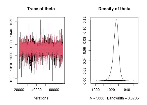
plot(MCMC2)
The output of the function
combinationWithOutliers_Gauss()
is a Markov chain of the
posterior distribution of the Bayesian model.
Here we will focus on the posterior distribution of the date of interest i.e. the parameter ’theta*.
MCMCSample2 <- cbind(MCMC2[[1]], MCMC2[[2]])
MCMCEvent2 <- as_events(MCMCSample2, calendar = CE())
plot(MCMCEvent2[, 1], level = 0.95)
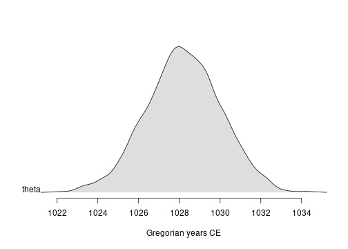
(M2 <- summary(MCMCEvent2[, 1], level = 0.95))
#> mad mean sd min q1 median q3 max start end
#> theta 1028 1028 3 1022 1027 1028 1029 1035 1025 1032
The date (mean posterior distribution) of the sunspot, estimated using a simple Bayesian model that combines dates and allows for outliers, is dates at 1028 years after Christ. This date is associated with a 95% confidence interval : [1025, 1032].
Let’s now use the function
combinationWithRandomEffect_Gauss()
.
<- combinationWithRandomEffect_Gauss(
MCMC3 M = sunspot$Age[1:5],
s = sunspot$Error[1:5],
refYear = rep(2016, 5),
studyPeriodMin = 0,
studyPeriodMax = 1500,
variable.names = c('theta')
)#> [1] "Update period"
#>
|
| | 0%
|
|* | 2%
|
|** | 4%
|
|*** | 6%
|
|**** | 8%
|
|***** | 10%
|
|****** | 12%
|
|******* | 14%
|
|******** | 16%
|
|********* | 18%
|
|********** | 20%
|
|*********** | 22%
|
|************ | 24%
|
|************* | 26%
|
|************** | 28%
|
|*************** | 30%
|
|**************** | 32%
|
|***************** | 34%
|
|****************** | 36%
|
|******************* | 38%
|
|******************** | 40%
|
|********************* | 42%
|
|********************** | 44%
|
|*********************** | 46%
|
|************************ | 48%
|
|************************* | 50%
|
|************************** | 52%
|
|*************************** | 54%
|
|**************************** | 56%
|
|***************************** | 58%
|
|****************************** | 60%
|
|******************************* | 62%
|
|******************************** | 64%
|
|********************************* | 66%
|
|********************************** | 68%
|
|*********************************** | 70%
|
|************************************ | 72%
|
|************************************* | 74%
|
|************************************** | 76%
|
|*************************************** | 78%
|
|**************************************** | 80%
|
|***************************************** | 82%
|
|****************************************** | 84%
|
|******************************************* | 86%
|
|******************************************** | 88%
|
|********************************************* | 90%
|
|********************************************** | 92%
|
|*********************************************** | 94%
|
|************************************************ | 96%
|
|************************************************* | 98%
|
|**************************************************| 100%
#> [1] "Acquire period"
#>
|
| | 0%
|
|* | 2%
|
|** | 4%
|
|*** | 6%
|
|**** | 8%
|
|***** | 10%
|
|****** | 12%
|
|******* | 14%
|
|******** | 16%
|
|********* | 18%
|
|********** | 20%
|
|*********** | 22%
|
|************ | 24%
|
|************* | 26%
|
|************** | 28%
|
|*************** | 30%
|
|**************** | 32%
|
|***************** | 34%
|
|****************** | 36%
|
|******************* | 38%
|
|******************** | 40%
|
|********************* | 42%
|
|********************** | 44%
|
|*********************** | 46%
|
|************************ | 48%
|
|************************* | 50%
|
|************************** | 52%
|
|*************************** | 54%
|
|**************************** | 56%
|
|***************************** | 58%
|
|****************************** | 60%
|
|******************************* | 62%
|
|******************************** | 64%
|
|********************************* | 66%
|
|********************************** | 68%
|
|*********************************** | 70%
|
|************************************ | 72%
|
|************************************* | 74%
|
|************************************** | 76%
|
|*************************************** | 78%
|
|**************************************** | 80%
|
|***************************************** | 82%
|
|****************************************** | 84%
|
|******************************************* | 86%
|
|******************************************** | 88%
|
|********************************************* | 90%
|
|********************************************** | 92%
|
|*********************************************** | 94%
|
|************************************************ | 96%
|
|************************************************* | 98%
|
|**************************************************| 100%
plot(MCMC3)
The output of the function
combinationWithRandomEffect_Gauss()
is a Markov chain of
the posterior distribution of the Bayesian model.
Here we will focus on the posterior distribution of the date of interest i.e. the parameter ’theta*.
MCMCSample3 <- cbind(MCMC3[[1]], MCMC3[[2]])
MCMCEvent3 <- as_events(MCMCSample3, calendar = CE())
plot(MCMCEvent3[, 1], level = 0.95)
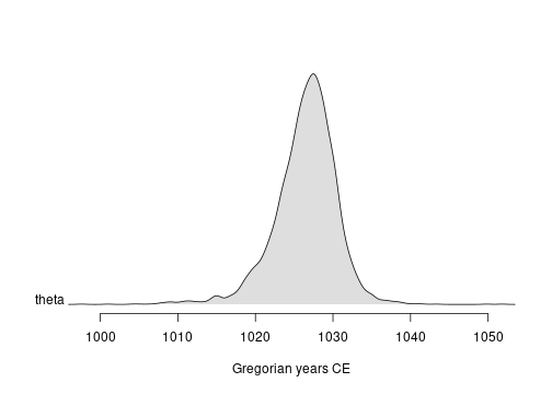
(M3 <- summary(MCMCEvent3[, 1], level = 0.95))
#> mad mean sd min q1 median q3 max start end
#> theta 1027 1026 5 998 1024 1027 1029 1052 1018 1033
The date (mean posterior distribution) of the sunspot, estimated using a simple Bayesian model that combines dates and allows for random effects, is dates at 1026 years after Christ. This date is associated with a 95% confidence interval : [1018, 1033].
If we want to date that event, we can use the Event model for combining Gaussian dates. In that example, we will investigate the posterior distribution of the date of the event (called ’theta*) and the posterior distribution of the dates associated with this event.
Finally, let’s use the function eventModel_Gauss()
and
the first 10 dates of the dataset sunspot. The study period should be
given in calendar year (BC/AD).
<- eventModel_Gauss(
MCMC4 M = sunspot$Age[1:5],
s = sunspot$Error[1:5],
refYear = rep(2016, 5),
studyPeriodMin = 900,
studyPeriodMax = 1500,
variable.names = c('theta', 'mu')
)#> [1] "Update period"
#>
|
| | 0%
|
|* | 2%
|
|** | 4%
|
|*** | 6%
|
|**** | 8%
|
|***** | 10%
|
|****** | 12%
|
|******* | 14%
|
|******** | 16%
|
|********* | 18%
|
|********** | 20%
|
|*********** | 22%
|
|************ | 24%
|
|************* | 26%
|
|************** | 28%
|
|*************** | 30%
|
|**************** | 32%
|
|***************** | 34%
|
|****************** | 36%
|
|******************* | 38%
|
|******************** | 40%
|
|********************* | 42%
|
|********************** | 44%
|
|*********************** | 46%
|
|************************ | 48%
|
|************************* | 50%
|
|************************** | 52%
|
|*************************** | 54%
|
|**************************** | 56%
|
|***************************** | 58%
|
|****************************** | 60%
|
|******************************* | 62%
|
|******************************** | 64%
|
|********************************* | 66%
|
|********************************** | 68%
|
|*********************************** | 70%
|
|************************************ | 72%
|
|************************************* | 74%
|
|************************************** | 76%
|
|*************************************** | 78%
|
|**************************************** | 80%
|
|***************************************** | 82%
|
|****************************************** | 84%
|
|******************************************* | 86%
|
|******************************************** | 88%
|
|********************************************* | 90%
|
|********************************************** | 92%
|
|*********************************************** | 94%
|
|************************************************ | 96%
|
|************************************************* | 98%
|
|**************************************************| 100%
#> [1] "Acquire period"
#>
|
| | 0%
|
|* | 2%
|
|** | 4%
|
|*** | 6%
|
|**** | 8%
|
|***** | 10%
|
|****** | 12%
|
|******* | 14%
|
|******** | 16%
|
|********* | 18%
|
|********** | 20%
|
|*********** | 22%
|
|************ | 24%
|
|************* | 26%
|
|************** | 28%
|
|*************** | 30%
|
|**************** | 32%
|
|***************** | 34%
|
|****************** | 36%
|
|******************* | 38%
|
|******************** | 40%
|
|********************* | 42%
|
|********************** | 44%
|
|*********************** | 46%
|
|************************ | 48%
|
|************************* | 50%
|
|************************** | 52%
|
|*************************** | 54%
|
|**************************** | 56%
|
|***************************** | 58%
|
|****************************** | 60%
|
|******************************* | 62%
|
|******************************** | 64%
|
|********************************* | 66%
|
|********************************** | 68%
|
|*********************************** | 70%
|
|************************************ | 72%
|
|************************************* | 74%
|
|************************************** | 76%
|
|*************************************** | 78%
|
|**************************************** | 80%
|
|***************************************** | 82%
|
|****************************************** | 84%
|
|******************************************* | 86%
|
|******************************************** | 88%
|
|********************************************* | 90%
|
|********************************************** | 92%
|
|*********************************************** | 94%
|
|************************************************ | 96%
|
|************************************************* | 98%
|
|**************************************************| 100%
The output of the eventModel_Gauss()
is the Markov chain
of the posterior distribution.
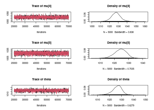
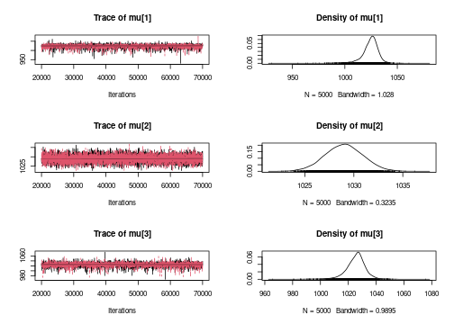
First, let’s check the convergence of the Markov chain of each parameter.
plot(MCMC4)
gelman.diag(MCMC4)
#> Potential scale reduction factors:
#>
#> Point est. Upper C.I.
#> mu[1] 1 1
#> mu[2] 1 1
#> mu[3] 1 1
#> mu[4] 1 1
#> mu[5] 1 1
#> theta 1 1
#>
#> Multivariate psrf
#>
#> 1
The Gelman diagnotic gives point estimates about 1, so convergence is reached.
Here we will focus on the posterior distribution of the event of interest (parameter ’theta*).
MCMCSample4 <- cbind(MCMC4[[1]], MCMC4[[2]])
MCMCEvent4 <- as_events(MCMCSample4, calendar = CE())
plot(MCMCEvent4[, 6], level = 0.95)
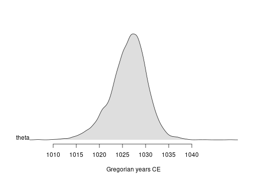
(M4 <- summary(MCMCEvent4[, 6], level = 0.95))
#> mad mean sd min q1 median q3 max start end
#> theta 1027 1026 5 1007 1024 1027 1029 1048 1018 1034
The date (mean posterior distribution) of the sunspot, estimated using a simple Bayesian model that combines dates and allows for individual random effects, is dates at 1026 years after Christ. This date is associated with a 95% confidence interval : [1018, 1034].