Plots credible intervals or HPD regions of a series of events.
Usage
# S4 method for class 'MCMC,missing'
plot(
  x,
  calendar = get_calendar(),
  density = TRUE,
  interval = NULL,
  level = 0.95,
  sort = TRUE,
  decreasing = TRUE,
  main = NULL,
  sub = NULL,
  ann = graphics::par("ann"),
  axes = TRUE,
  frame.plot = FALSE,
  panel.first = NULL,
  panel.last = NULL,
  col.density = "grey",
  col.interval = "#77AADD",
  ...
)
Arguments
- x
An
MCMCobject.- calendar
A
aion::TimeScaleobject specifying the target calendar (seecalendar()).- density
A
logicalscalar: should estimated density be plotted?- interval
A
characterstring specifying the confidence interval to be drawn. It must be one of "credible" (credible interval) or "hdr" (highest posterior density interval). Any unambiguous substring can be given. IfNULL(the default) no interval is computed.- level
A length-one
numericvector giving the confidence level.- sort
A
logicalscalar: should the data be sorted?- decreasing
A
logicalscalar: should the sort order be decreasing? Only used ifsortisTRUE.- main
A
characterstring giving a main title for the plot.- sub
A
characterstring giving a subtitle for the plot.- ann
A
logicalscalar: should the default annotation (title and x and y axis labels) appear on the plot?- axes
A
logicalscalar: should axes be drawn on the plot?- frame.plot
A
logicalscalar: should a box be drawn around the plot?- panel.first
An an
expressionto be evaluated after the plot axes are set up but before any plotting takes place. This can be useful for drawing background grids.- panel.last
An
expressionto be evaluated after plotting has taken place but before the axes, title and box are added.- col.density, col.interval
A specification for the plotting colors.
- ...
Extra parameters to be passed to
stats::density().
Value
plot() is called it for its side-effects: it results in a graphic being
displayed (invisibly returns x).
See also
Other plot methods:
plot_phases
Examples
## Coerce to MCMC
eve <- as_events(mcmc_events, calendar = CE(), iteration = 1)
## Summary
summary(eve, calendar = CE())
#> mad mean sd min q1 median q3 max start end
#> E1 -900 -638 272 -1349 -889 -658 -386 -5 -1046 -202
#> E2 -1766 -1785 100 -2000 -1857 -1785 -1719 -971 -1981 -1611
#> E3 -702 -656 92 -1229 -717 -672 -611 -67 -803 -450
#> E4 -1241 -1236 87 -1864 -1289 -1235 -1181 -719 -1401 -1064
summary(eve, calendar = BP())
#> mad mean sd min q1 median q3 max start end
#> E1 2850 2588 1680 3299 2839 2608 2338 1957 2998 2154
#> E2 3716 3737 1852 3950 3807 3735 3671 2923 3933 3561
#> E3 2652 2608 1860 3181 2667 2624 2561 2017 2753 2400
#> E4 3191 3186 1863 3814 3239 3187 3131 2669 3351 3016
## Plot events
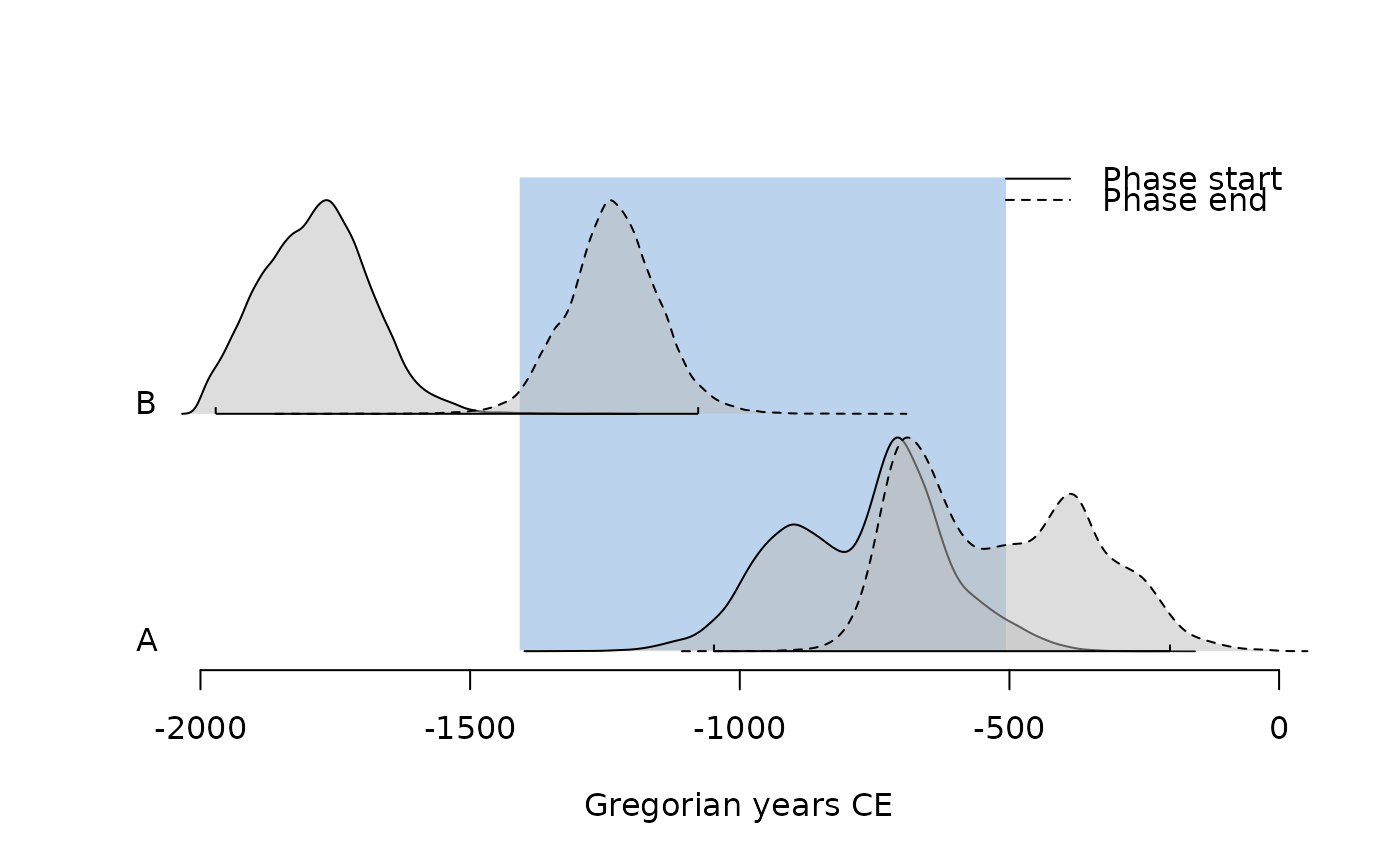
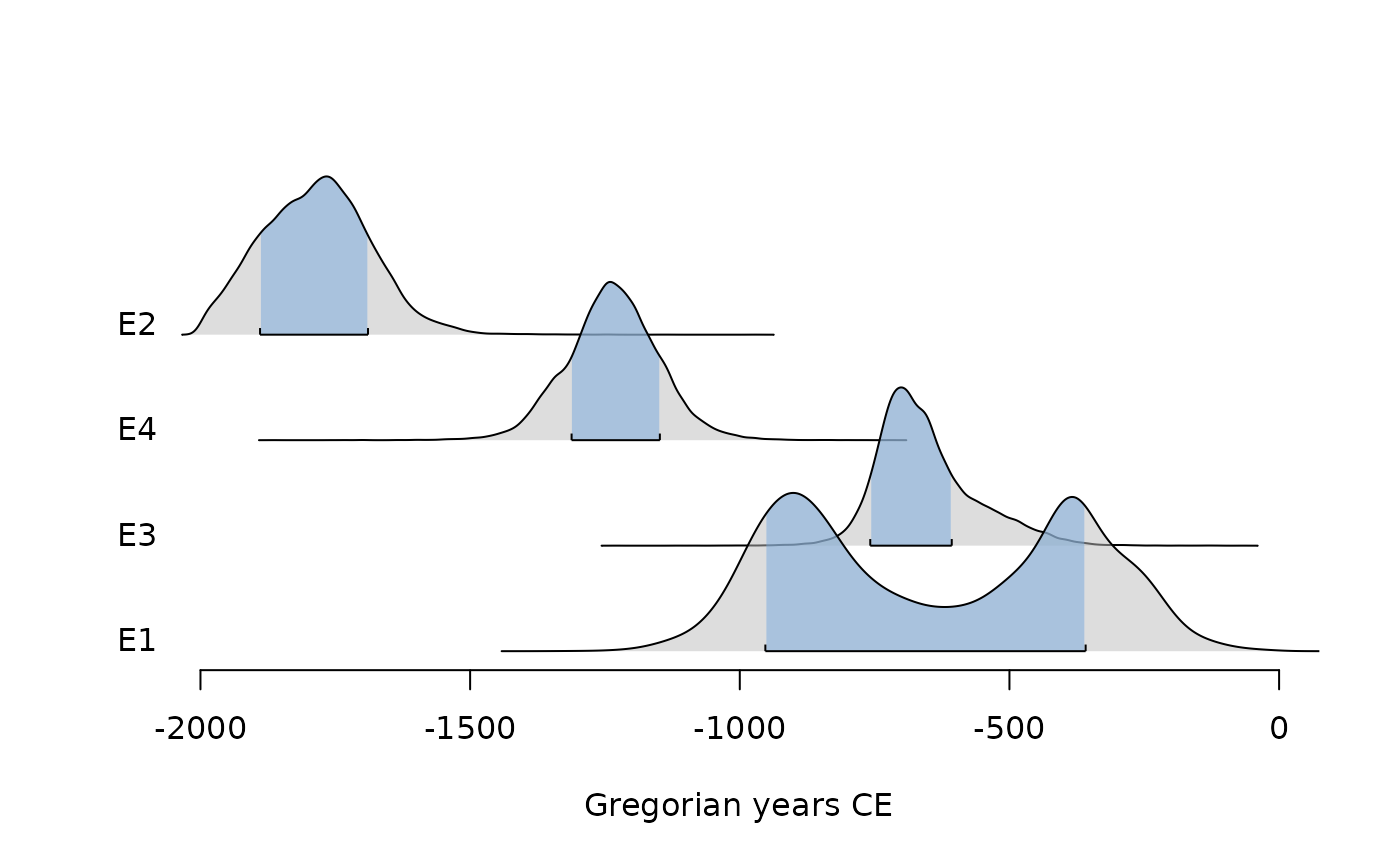
plot(eve, calendar = CE(), interval = "credible", level = 0.68)
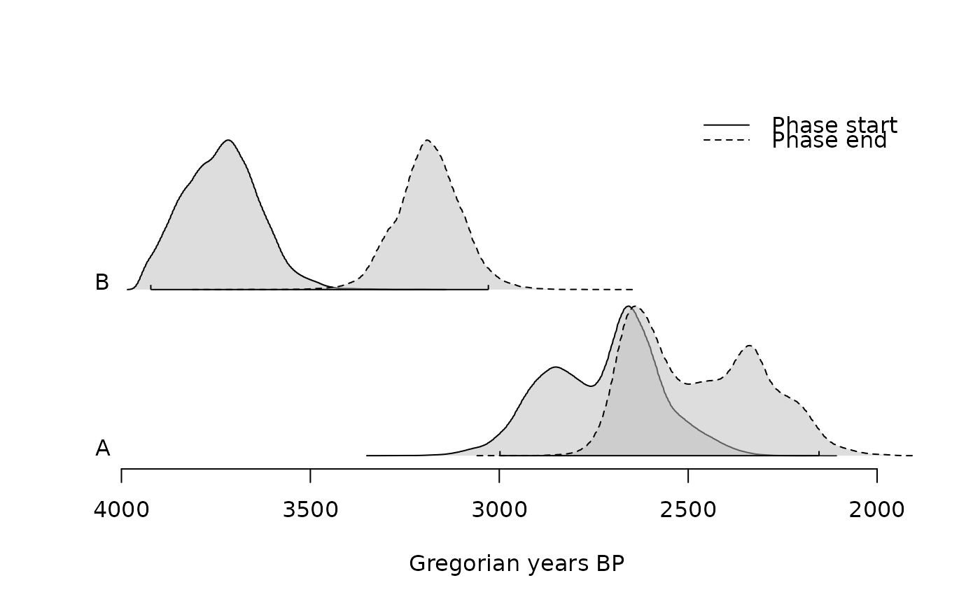
 plot(eve, calendar = BP(), interval = "hdr", level = 0.68)
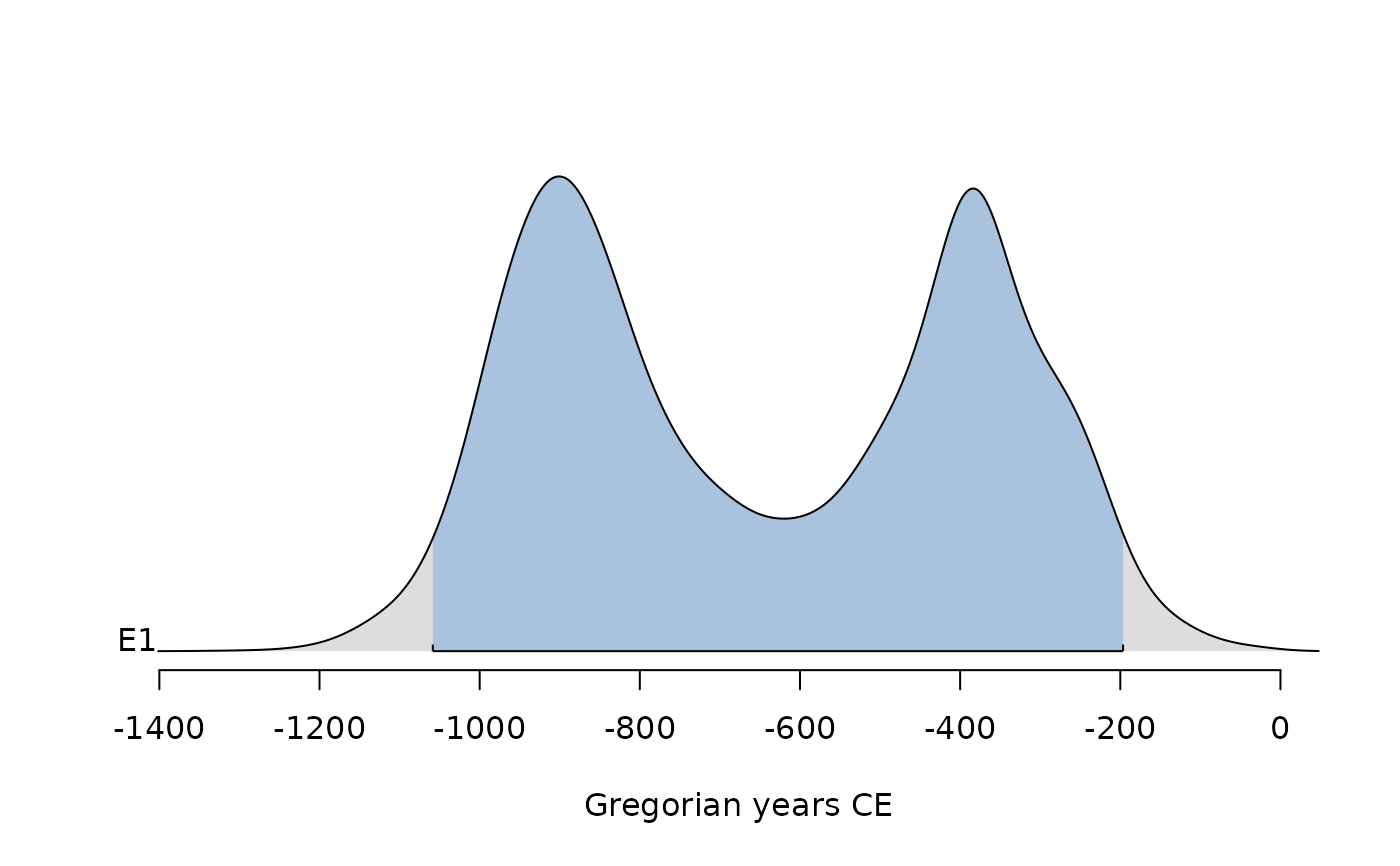
 plot(eve[, 1], interval = "hdr")
 ## Compute phases
pha <- phases(eve, groups = list(B = c(2, 4), A = c(1, 3)))
## Summary
summary(pha, calendar = CE())
#> $B
#> mad mean sd min q1 median q3 max start end
#> start -1766 -1785 100 -2000 -1857 -1785 -1719 -1223 -1981 -1611
#> end -1240 -1235 87 -1833 -1289 -1235 -1181 -719 -1404 -1067
#> duration 561 551 132 5 464 552 639 1157 297 806
#>
#> $A
#> mad mean sd min q1 median q3 max start end
#> start -708 -773 148 -1349 -890 -749 -671 -207 -1059 -501
#> end -690 -521 169 -1050 -670 -537 -384 -5 -776 -214
#> duration 278 253 138 1 151 249 345 880 1 487
#>
summary(pha, calendar = BP())
#> $B
#> mad mean sd min q1 median q3 max start end
#> start 3718 3737 1852 3950 3807 3735 3671 3173 3933 3561
#> end 3192 3187 1863 3783 3239 3187 3131 2669 3354 3019
#> duration 1391 1401 1820 1945 1488 1398 1311 793 1653 1146
#>
#> $A
#> mad mean sd min q1 median q3 max start end
#> start 2660 2723 1802 3299 2840 2701 2623 2157 3011 2453
#> end 2640 2473 1783 3000 2622 2487 2334 1957 2726 2166
#> duration 1674 1699 1814 1949 1801 1703 1607 1072 1949 1465
#>
## Plot phases
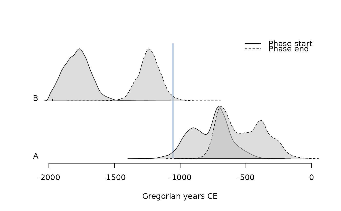
plot(pha, calendar = BP())
## Compute phases
pha <- phases(eve, groups = list(B = c(2, 4), A = c(1, 3)))
## Summary
summary(pha, calendar = CE())
#> $B
#> mad mean sd min q1 median q3 max start end
#> start -1766 -1785 100 -2000 -1857 -1785 -1719 -1223 -1981 -1611
#> end -1240 -1235 87 -1833 -1289 -1235 -1181 -719 -1404 -1067
#> duration 561 551 132 5 464 552 639 1157 297 806
#>
#> $A
#> mad mean sd min q1 median q3 max start end
#> start -708 -773 148 -1349 -890 -749 -671 -207 -1059 -501
#> end -690 -521 169 -1050 -670 -537 -384 -5 -776 -214
#> duration 278 253 138 1 151 249 345 880 1 487
#>
summary(pha, calendar = BP())
#> $B
#> mad mean sd min q1 median q3 max start end
#> start 3718 3737 1852 3950 3807 3735 3671 3173 3933 3561
#> end 3192 3187 1863 3783 3239 3187 3131 2669 3354 3019
#> duration 1391 1401 1820 1945 1488 1398 1311 793 1653 1146
#>
#> $A
#> mad mean sd min q1 median q3 max start end
#> start 2660 2723 1802 3299 2840 2701 2623 2157 3011 2453
#> end 2640 2473 1783 3000 2622 2487 2334 1957 2726 2166
#> duration 1674 1699 1814 1949 1801 1703 1607 1072 1949 1465
#>
## Plot phases
plot(pha, calendar = BP())
 plot(pha, succession = "hiatus")
 plot(pha, succession = "transition")